Example Workflow for Data Standardization and Analysis Reproducibility

Here we document an example of how we 1. standardized data into a community-accepted standard (NWB) and 2. enabled reproducibility of paper figures as a starting point for secondary analyses.

In doing this exercise, we complete a pipeline that is key for any datasets that are uploaded to EMBER. It is important that not only is the data standardized for improved storage and metadata retrieval, but that the standardized data can also be used for secondary processing and analyses. Reproducing key figures is the first such verification step towards ensuring that open datasets can be repurposed for new scientific endeavours.

Public Products

1. Conversion script from the original processed data files to a single NWB
2. Jupyter notebook to recreate paper figures from the NWB file

Original dataset

The original dataset is associated with the paper Human neural dynamics of real-world and imagined navigation, authored by a BBQS Team (Dr. Nanthia Suthana, PI). It contains four .mat files containing highly processed data for each of the four figures of the paper. In addition, the MATLAB codes to generate each figure are comprised of four .m files.

Conversion

In collaboration with Dr. Suthana and Dr. Seeber (lead author), we explored each of the data variables in the original .mat files and identified analogous containers within the NWB file structure.

Most of the data variables are relevant to multiple subjects at the same time (e.g., group averages).

Because of this, we opted to convert the data into an NWB extension: ndx-multisubjects. In addition to group averages, this extension is also suitable for storing sensor data that encompasses multiple subjects at once (e.g., video of multiple subjects in an environment, microphone data capturing audio from multiple sources, etc).

Each variable within the .mat files was then converted into the appropriate modality type within NWB with the relevant metadata capture (sampling rates, start times, descriptions of variables).

Each variable of the four .mat files was converted into a container within a single NWB file

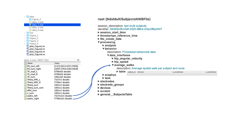
The current version of the conversion script is located at https://github.com/brain-bbqs/reproforce/blob/main/suthana/Suthana_Zenodo_Conversion.py.

Verfication

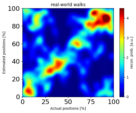
To verify that the original data was properly converted into NWB, we checked whether the NWB data could be used to replicate the MATLAB code and resulting figures.

We were able to recreate all figures from the original paper.

The current notebook for recreating figures is located at https://github.com/brain-bbqs/reproforce/blob/main/suthana/create_figs_Zenodo.ipynb.

Below are a few examples:

Fig. 1 Original

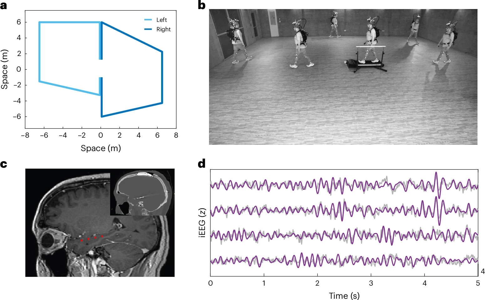
Fig. 1d recreated in Python with NWB data

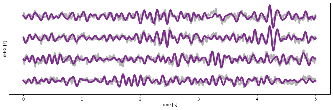
Fig 2. Original

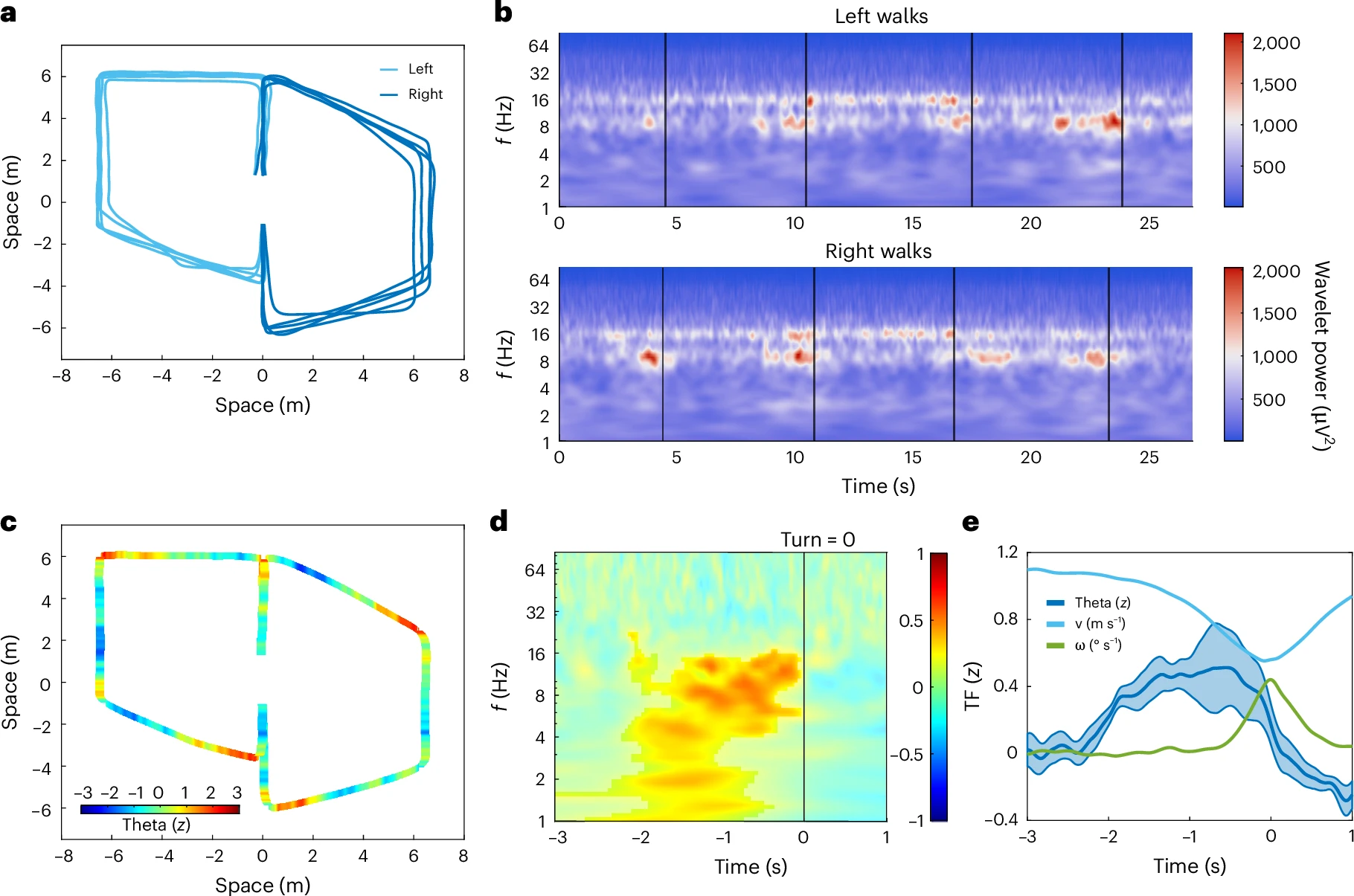
Fig. 2b top recreated in Python with NWB data

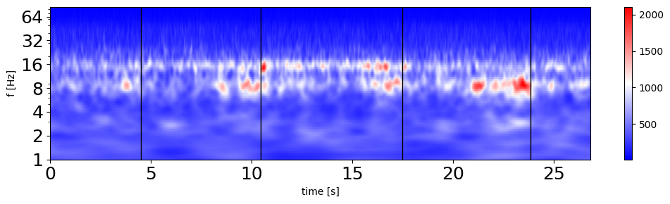
Fig. 3 Original

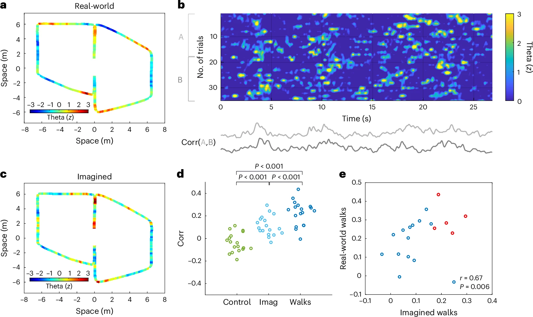
Fig. 3a recreated in Python with NWB data

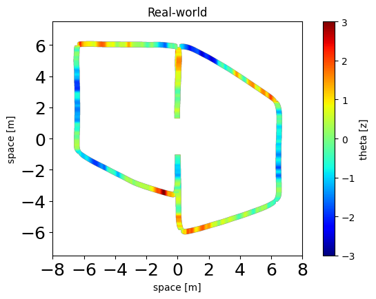
Fig. 4 Original

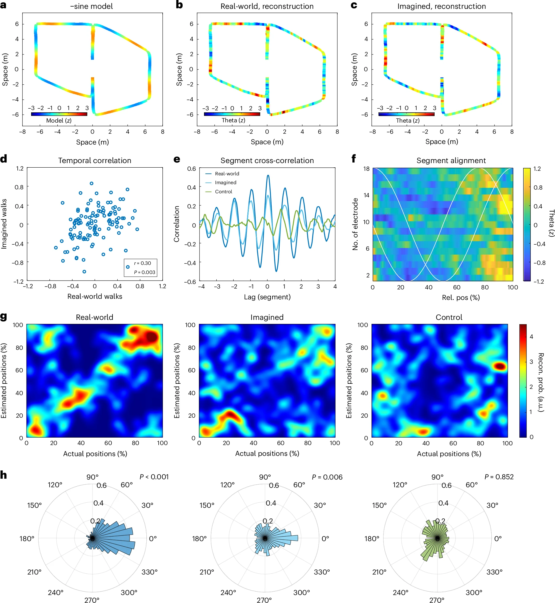
Fig. 4g recreated in Python with NWB data

Next Steps

As mentioned above, the first step towards enabling robust secondary analyses is to replicate publication figures or analyses produced with the original file format.

To continue towards this effort, the following next steps are outlined to enable novel analyses that are best served with the richness of raw data.

• once final reviews of the converted Zenodo data are complete, upload the NWB file as a version 2 of the Zenodo dataset (with permissions from Dr. Seeber and Dr. Suthana)
• convert original raw data into NWB
• replicate analyses from the original raw data stored in NWB, using the processed Zenodo data as an intermediate check
• perform secondary (new) analyses